My first encounter with C++ was way back in the 1990s, when it was one of the Real Programming Languages that I sometimes heard about as I was still splashing about in the kiddie pool with Visual Basic, PHP and JavaScript. The first formally standardized version of C++ is the ISO 1998 standard, but it had been making headways as a ‘better C’ for decades at that point since Bjarne Stroustrup added that increment operator to C in 1979 and released C++ to the public in 1985.
Why did I pick C++ as my primary programming language? Mainly because it was well supported and with free tooling: a free Borland compiler or g++ on the GCC side. Alternatives like VB, Java, and D felt far too niche compared to established languages, while C++ gave you access to the lingua franca of C while adding many modern features like OOP and a more streamlined syntax in addition to the Standard Template Library (STL) with gobs of useful building blocks.
Years later, as a grizzled senior C++ developer, I have come to embrace the notion that being good at a programming language also means having strong opinions on all that is wrong with the language. True to form, while C++ has many good points, there are still major warts and many heavily neglected aspects that get me and other C++ developers riled up.
Why We Fell In Love
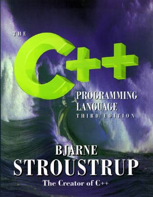 Cover of the third edition of The C++ Programming Language by Bjarne Stroustrup.
What frightened me about C++ initially was just how big and scary it seemed, with gargantuan IDEs like Microsoft’s Visual Studio, complex build systems, and graphical user interface that seemed to require black magic far beyond my tiny brain’s comprehension. Although using the pure C-based Win32 API does indeed require ritual virgin sacrifices, and Windows developers only talk about MFC when put under extreme duress, the truth is that C++ itself is rather simple, and writing complex applications is easy once you break it down into steps. For me the breakthrough came after buying a copy of Stroustrup’s The C++ Programming Language, specifically the third edition that covered the C++98 standard.
More than just a reference, it laid out clearly for me not only how to write basic C++ programs, but also how to structure my code and projects, as well as the reasonings behind each of these aspects. For many years this book was my go-to resource, as I developed my rudimentary, scripting language-afflicted skills into something more robust.
Probably the best part about C++ is its flexibility. It never limits you to a single programming paradigm, while it gives you the freedom to pick the desire path of your choice. Although an astounding number of poor choices can be made here, with a modicum of care and research you do not have to end up hoisted with your own petard. Straying into the C-compatibility part of C++ is especially fraught with hazards, but that’s why we have the C++ bits so that we don’t have to touch those.
Reflecting With C++11
It would take until 2011 for the first major update to the C++ standard, by which time I had been using C++ mostly for increasingly more elaborate hobby projects. But then I got tossed into a number of commercial C and C++ projects that would put my burgeoning skills to the test. Around this time I found the first major items in C++ that are truly vexing.
Common issues like header-include order and link order, which can lead to circular dependencies, are some of such truly delightful aspects. The former is mostly caused by the rather simplistic way that header files are just slapped straight into the source code by the preprocessor. Like in C, the preprocessor simply looks at your #include "widget/foo.h" and replaces it with the contents of foo.h with absolutely no consideration for side effects and cases of spontaneous combustion.
Along the way, further preprocessor statements further mangle the code in happy-fun ways, which is why the GCC g++ and compatible compilers like Clang have the -E flag to only run the preprocessor so that you can inspect the preprocessed barf that was going to be sent to the compiler prior to it violently exploding. The trauma suffered here is why I heartily agree with Mr. Stroustrup that the preprocessor is basically evil and should only be used for the most basic stuff like includes, very simple constants and selective compilation. Never try to be cute or smart with the preprocessor or whoever inherits your codebase will find you.
If you got your code’s architectural issues and header includes sorted out, you’ll find that C++’s linker is just as dumb as that of C. After being handed the compiled object files and looking at the needed symbols, it’ll waddle into the list of libraries, look at each one in order and happily ignore previously seen symbols if they’re needed later. You’ll suffer for this with tools like ldd and readelf as you try to determine whether you are just dense, the linker is dense or both are having buoyancy issues.
These points alone are pretty traumatic, but you learn to cope with them like you cope with a gaggle of definitely teething babies a few rows behind you on that transatlantic flight. The worst part is probably that neither C++11 nor subsequent standards have addressed either to any noticeable degree, with a shift from C-style compile units to Ada-like modules probably never going to happen.
The ‘modules at home‘ feature introduced with C++20 are effectively just limited C-style headers without the preprocessor baggage, without the dependency analysis and other features that make languages like Ada such a joy to build code with.
Non-Deterministic Initialization
Although C++ and C++11 in particular removes a lot of undefined behavior that C is infamous for, there are still many parts where expected behavior is effectively random or at least platform-specific. One such example is that of static initialization, officially known as the Static initialization order fiasco. Essentially what it means is that you cannot count on a variable declared static to be initialized during general initialization between different compile units.
This also affects the same compile units when you are initializing a static std::map instance with data during initialization, as I learned the hard way during a project when I saw random segmentation faults on start-up related to the static data structure instance. The executive summary here is that you should not assume that anything has been implicitly initialized during application startup, and instead you should do explicit initialization for such static structures.
An example of this can be found in my NymphRPC project, in which I used this same solution to prevent initialization crashes. This involves explicitly creating the static map rather than praying that it gets created in time:
static map<UInt32, NymphMethod*> &methodsIdsStatic = NymphRemoteClient::methodsIds();
With the methodsIds() function:
map<UInt32, NymphMethod*>& NymphRemoteClient::methodsIds() {
static map<UInt32, NymphMethod*>* methodsIdsStatic = new map<UInt32, NymphMethod*>();
return *methodsIdsStatic;
}
It are these kind of niggles along with the earlier covered build-time issues that tend to sap a lot of time during development until you learn to recognize them in advance along with fixes.
Fading Love
Don’t get me wrong, I still think that C++ is a good programming language at its core, it is just that it has those rough spots and sharp edges that you wish weren’t there. There is also the lack of improvements to some rather fundamental aspects in the STL, such as the unloved C++ string library. Compared to Ada standard library strings, the C++ STL string API is very barebones, with a lot of string manipulation requiring writing the same tedious code over and over as convenience functions are apparently on nobody’s wish list.
One good thing that C++11 brought to the STL was multi-tasking support, with threads, mutexes and so on finally natively available. It’s just a shame that its condition variables are plagued by spurious wake-ups and a more complicated syntax than necessary. This gets even worse with the Filesystem library that got added in C++17. Although it’s nice to have more than just basic file I/O in C++ by default, it is based on the library in Boost, which uses a coding style, type encapsulation obsession, and abuse of namespaces that you apparently either love or hate.
I personally have found the POCO C++ libraries to be infinitely easier to use, with a relatively easy to follow implementation. I even used the POCO libraries for the NPoco project, which adapts the code to microcontroller use and adds FreeRTOS support.
Finally, there are some core language changes that I fundamentally disagree with, such as the addition of type inference with the auto keyword outside of templates, which is a weakly typed feature. As if it wasn’t bad enough to have the chaos of mixed explicit and implicit type casting, now we fully put our faith into the compiler, pray nobody updates code elsewhere that may cause explosions later on, and remove any type-related cues that could be useful to a developer reading the code.
But at least we got constexpr, which is probably incredibly useful to people who use C++ for academic dissertations rather than actual programming.
Hope For The Future
I’ll probably keep using C++ for the foreseeable future, while grumbling about all of ’em whippersnappers adding useless things that nobody was asking for. Since the general take on adding new features to C++ is that you need to do all the legwork yourself – like getting into the C++ working groups to promote your feature(s) – it’s very likely that few actually needed features will make it into new C++ standards, as those of us who are actually using the language are too busy doing things like writing production code in it, while simultaneously being completely disinterested in working group politics.
Fortunately there is excellent backward compatibility in C++, so those of us in the trenches can keep using the language any way we like along with all the patches we wrote to ease the pains. It’s just sad that there’s now such a split forming between C++ developers and C++ academics.
It’s one of the reasons why I have felt increasingly motivated over the past years to seek out other languages, with Ada being one of my favorites. Unlike C++, it doesn’t have the aforementioned build-time issues, and while its super-strong type system makes getting started with writing the business logic slower, it prevents so many issues later on, along with its universal runtime bounds checking. It’s not often that using a programming language makes me feel something approaching joy.
Giving up on a programming language with which you quite literally grew up is hard, but as in any relationship you have to be honest about any issues, no matter whether it’s you or the programming language. That said, maybe some relationship counseling will patch things up again in the future, with us developers are once again involved in the language’s development.
From Blog – Hackaday via this RSS feed


.jpg)